Εφαρμογή DFT: Θεμελιώδης Κατάσταση Ατόμου Ne
1. Εισαγωγή
Σε αυτή την άσκηση στόχος μας είναι να υπολογίσουμε την κατάσταση ελάχιστης ενέργειας (ground state) του ατόμου Neon χρησιμοποιώντας τον αλγόριθμο DFT.
2. Κώδικας
import numpy as np
import matplotlib.pyplot as plt
from scipy.linalg import solve_banded, eigh_tridiagonal

# ─────────────────────────────────────────────
# Radial grid
# ─────────────────────────────────────────────
rmax = 65.0
dr   = 0.015
r    = np.arange(dr/2, rmax + dr/2, dr)
N    = len(r)
vol  = 4 * np.pi * r**2

# ─────────────────────────────────────────────
# Atomic number: Neon Z=10, 10 electrons
# occupying 1s² 2s² 2p⁶
# ─────────────────────────────────────────────
Z        = 10.0
N_elec   = 10
N_orb    = 3
occ      = [2, 2, 6]

# ─────────────────────────────────────────────
# Kinetic energy (Laplacian)
# ─────────────────────────────────────────────
laplacian_diag = -2.0 * np.ones(N)     / dr**2
laplacian_off  =  1.0 * np.ones(N - 1) / dr**2

# ─────────────────────────────────────────────
# Poisson solver matrix
# ─────────────────────────────────────────────
poisson_diag   =  2.0 * np.ones(N)     / dr**2
poisson_off    = -1.0 * np.ones(N - 1) / dr**2
poisson_banded = np.vstack([
    np.hstack((0, poisson_off)),
    poisson_diag,
    np.hstack((poisson_off, 0))
])

# ─────────────────────────────────────────────
# Initial electron density for Ne (10 electrons)
# ─────────────────────────────────────────────
n = (N_elec / (4 * np.pi)) * (Z**3 / 8) * np.exp(-Z * r)
n = np.clip(n, 1e-30, None)

# ─────────────────────────────────────────────
# LDA (Perdew-Zunger 1981) parameters
# ─────────────────────────────────────────────
A      =  0.0311
B      = -0.048
C      =  0.002
D      = -0.0116
gamma  = -0.1423
beta1  =  1.0529
beta2  =  0.3334

def get_Vxc(n):
    """LDA exchange-correlation potential (Perdew-Zunger 1981)."""
    n_safe = np.clip(n, 1e-30, None)
    rs = (3.0 / (4.0 * np.pi * n_safe))**(1.0/3.0)
    Vx = -(3.0 / np.pi * n_safe)**(1.0/3.0)
    Vc = np.where(
        rs < 1,
        A*np.log(rs) + B + C*rs*np.log(rs) + D*rs
            - rs/3.0 * (A/rs + C*np.log(rs) + C + D),
        gamma*(1 + 7.0/6.0*beta1*np.sqrt(rs) + 4.0/3.0*beta2*rs)
            / (1 + beta1*np.sqrt(rs) + beta2*rs)**2
    )
    return Vx + Vc

def get_eps_xc(n):
    """LDA exchange-correlation energy density (Perdew-Zunger 1981)."""
    n_safe = np.clip(n, 1e-30, None)
    rs_ec = (3.0 / (4.0 * np.pi * n_safe))**(1.0/3.0)
    eps_x = -0.75 * (3.0 / np.pi * n_safe)**(1.0/3.0)
    eps_c = np.where(
        rs_ec < 1,
        A*np.log(rs_ec) + B + C*rs_ec*np.log(rs_ec) + D*rs_ec,
        gamma / (1 + beta1*np.sqrt(rs_ec) + beta2*rs_ec)
    )
    return eps_x, eps_c

# ─────────────────────────────────────────────
# SCF loop
# ─────────────────────────────────────────────
alpha    = 0.3
tol      = 1e-5
max_iter = 300

energy_history = []
E_ref_Ne = -128.5450  # Reference LDA energy for Ne (Ha)

print("SCF loop for Neon (Z=10, 1s² 2s² 2p⁶)\n")

for iteration in range(max_iter):

    # Hartree potential via Poisson equation
    rhs      = 4 * np.pi * r * n
    rhs[0]   = 0.0
    rhs[-1]  = N_elec
    U        = solve_banded((1, 1), poisson_banded, rhs)
    VH       = U / r

    # XC and effective potential
    Vxc  = get_Vxc(n)
    Vext = -Z / r
    Veff = Vext + VH + Vxc

    # Solve KS equation – get lowest N_orb orbitals
    diag = -0.5 * laplacian_diag + Veff
    off  = -0.5 * laplacian_off
    eps, eigvec = eigh_tridiagonal(
        diag, off,
        select='i', select_range=(0, N_orb - 1)
    )

    # Normalize orbitals and build new density
    orbitals = []
    n_new    = np.zeros(N)
    for i in range(N_orb):
        u_i  = eigvec[:, i]
        u_i /= np.sqrt(np.trapz(u_i**2, r))
        orbitals.append(u_i)
        n_new += occ[i] * u_i**2 / (4 * np.pi * r**2)

    # Energies
    eps_x_vals, eps_c_vals = get_eps_xc(n)
    Ts   = sum(occ[i]*eps[i] for i in range(N_orb)) - np.trapz(Veff * n * vol, r)
    EH   = 0.5 * np.trapz(VH          * n * vol, r)
    Ex   =       np.trapz(eps_x_vals  * n * vol, r)
    Ec   =       np.trapz(eps_c_vals  * n * vol, r)
    Eext =       np.trapz(Vext        * n * vol, r)
    Etot = Ts + EH + Ex + Ec + Eext
    energy_history.append(Etot)

    # Convergence check
    delta_n = np.max(np.abs(n_new - n))
    print(f"Iter {iteration+1:4d} | Etot = {Etot:.6f} Ha | "
          f"ε_1s = {eps[0]:.4f} | ε_2s = {eps[1]:.4f} | "
          f"ε_2p = {eps[2]:.4f} | Δn = {delta_n:.2e}")

    # Density mixing
    n = (1 - alpha) * n + alpha * n_new
    n = np.clip(n, 1e-30, None)

    if delta_n < tol:
        print(f"\nConverged in {iteration+1} iterations")
        print(f"  Final total energy : Etot  = {Etot:.6f} Ha")
        print(f"  Reference (LDA)    : E_Ne  = {E_ref_Ne:.6f} Ha")
        print(f"  Difference         : ΔE    = {abs(Etot - E_ref_Ne):.6f} Ha")
        print(f"  1s orbital energy  : ε_1s  = {eps[0]:.6f} Ha")
        print(f"  2s orbital energy  : ε_2s  = {eps[1]:.6f} Ha")
        print(f"  2p orbital energy  : ε_2p  = {eps[2]:.6f} Ha")
        break
else:
    print("Did not converge within max iterations!")

# ─────────────────────────────────────────────
# Plots
# ─────────────────────────────────────────────
fig, axes = plt.subplots(1, 3, figsize=(16, 5))

# Plot 1: KS orbitals
u_1s = orbitals[0]
u_2s = orbitals[1]
u_2p = orbitals[2]
axes[0].plot(r, u_1s, color='steelblue',  linewidth=2, label='1s')
axes[0].plot(r, u_2s, color='darkorange', linewidth=2, label='2s')
axes[0].plot(r, u_2p, color='green',      linewidth=2, label='2p')
axes[0].set_xlabel('r [Bohr]')
axes[0].set_ylabel('u(r) [a.u.]')
axes[0].set_title('KS Orbitals u(r)')
axes[0].set_xlim(0, 5)
axes[0].axhline(0, color='black', linewidth=0.5, linestyle='--')
axes[0].legend()
axes[0].grid(True, alpha=0.3)

# Plot 2: Electron density
axes[1].plot(r, vol * n, color='tomato', linewidth=2)
axes[1].set_xlabel('r [Bohr]')
axes[1].set_ylabel('4πr²n(r) [a.u.]')
axes[1].set_title('Electron Density n(r)')
axes[1].set_xlim(0, 5)
axes[1].grid(True, alpha=0.3)

# Plot 3: Energy convergence
axes[2].plot(range(1, len(energy_history)+1), energy_history,
             color='purple', linewidth=2, marker='o', markersize=3)
axes[2].axhline(y=E_ref_Ne, color='red', linestyle='--',
                linewidth=1.5, label=f'Reference: {E_ref_Ne} Ha')
axes[2].set_xlabel('SCF Iteration')
axes[2].set_ylabel('Total Energy [Ha]')
axes[2].set_title('Total Energy Convergence')
axes[2].legend()
axes[2].grid(True, alpha=0.3)

plt.suptitle('Neon Atom (Z=10) DFT Results',
             fontsize=14, fontweight='bold', y=1.02)
plt.tight_layout()
plt.show()

# ─────────────────────────────────────────────
# Diagnostics
# ─────────────────────────────────────────────
N_e_num = np.trapz(vol * n, r)
print(f"\nElectron Count Check: N_e = {N_e_num:.6f} (should be {N_elec})")
for i, u_i in enumerate(orbitals):
    norm = np.trapz(u_i**2, r)
    print(f"Normalization orbital {i+1}: {norm:.10f} (should be 1)")
3. Εξήγηση
3.1 Φυσικό Πρόβλημα
Στόχος της παρούσας εφαρμογής είναι ο υπολογισμός της θεμελιώδους κατάστασης του ατόμου Νέον (Ne) με ατομικό αριθμό Z = 10 χρησιμοποιώντας τη Θεωρία Density Functional Theory – DFT. Το άτομο του νέον διαθέτει δέκα ηλεκτρόνια τα οποία καταλαμβάνουν τα τροχιακά:
\[ 1s^2\,2s^2\,2p^6 \]
Η DFT επιτρέπει τον υπολογισμό των ηλεκτρονικών ιδιοτήτων ενός συστήματος μέσω της ηλεκτρονιακής πυκνότητας \(n(r)\), αποφεύγοντας την άμεση επίλυση του προβλήματος πολλών ηλεκτρονίων. Επειδή το άτομο είναι σφαιρικά συμμετρικό, όλες οι φυσικές ποσότητες εξαρτώνται μόνο από την ακτινική συντεταγμένη \(r\). Για τον λόγο αυτό το τρισδιάστατο πρόβλημα μετατρέπεται σε μονοδιάστατο ακτινικό πρόβλημα.
3.2 Κατασκευή Ακτινικού Πλέγματος
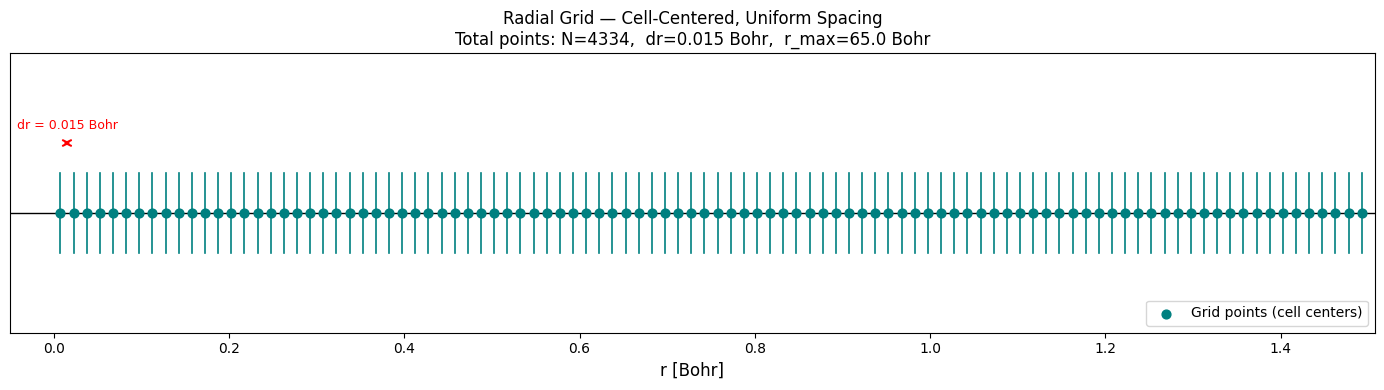
Το πρώτο βήμα του αλγορίθμου είναι η δημιουργία ενός ομοιόμορφου ακτινικού πλέγματος πάνω στο οποίο θα διακριτοποιηθούν οι εξισώσεις Kohn–Sham. Το πλέγμα ορίζεται από τις παραμέτρους:
\[ r_{\max}=65 \; \text{Bohr} \]
\[ \Delta r = 0.015 \; \text{Bohr} \]
Τα σημεία του πλέγματος τοποθετούνται σύμφωνα με τη σχέση:
\[ r_i=\left(i+\frac12\right)\Delta r \]
Η επιλογή αυτή αποφεύγει το σημείο \(r=0\), όπου το πυρηνικό δυναμικό Coulomb:
\[ V_{\text{ext}}(r)= -\frac{Z}{r} \]
παρουσιάζει μαθηματική ιδιομορφία. Με αυτόν τον τρόπο εξασφαλίζεται μεγαλύτερη αριθμητική σταθερότητα κατά την επίλυση των εξισώσεων.
3.3 Διακριτοποίηση του Τελεστή Laplace
Για την αριθμητική επίλυση των εξισώσεων Kohn–Sham απαιτείται η διακριτοποίηση της δεύτερης παραγώγου ως προς την ακτινική συντεταγμένη. Η προσέγγιση πραγματοποιείται με τη μέθοδο 3-point finite difference approximation.
Η δεύτερη παράγωγος της ακτινικής κυματοσυνάρτησης \(u(r)\) προσεγγίζεται από τη σχέση:
$$ \frac{d^2u}{dr^2} \approx \frac{u_{i+1}-2u_i+u_{i-1}} {\Delta r^2} $$
Η παραπάνω έκφραση χρησιμοποιεί τρία γειτονικά σημεία του πλέγματος: το προηγούμενο σημείο \(i-1\), το τρέχον σημείο \(i\) και το επόμενο σημείο \(i+1\).
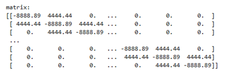
Η διακριτοποίηση οδηγεί σε έναν τριδιαγώνιο πίνακα της μορφής:
\[ \nabla^2 = \frac{1}{\Delta r^2} \begin{bmatrix} -2 & 1 & 0 & \cdots & 0 \\ 1 & -2 & 1 & \cdots & 0 \\ 0 & 1 & -2 & \cdots & 0 \\ \vdots & \vdots & \vdots & \ddots & 1 \\ 0 & 0 & 0 & 1 & -2 \end{bmatrix} \]
Στον πίνακα αυτό:
- Η κύρια διαγώνιος περιέχει την τιμή \(-2/\Delta r^2\).
- Οι δύο πλευρικές διαγώνιοι περιέχουν την τιμή \(+1/\Delta r^2\).
Για το συγκεκριμένο πλέγμα με:
\[ \Delta r = 0.015 \; \text{Bohr} \]
προκύπτουν οι αριθμητικές τιμές:
\[ -\frac{2}{(0.015)^2} = -8888.89 \]
\[ +\frac{1}{(0.015)^2} = 4444.44 \]
Ο πίνακας αυτός χρησιμοποιείται για την κατασκευή του τελεστή κινητικής ενέργειας των εξισώσεων Kohn–Sham:
\[ \hat{T} = -\frac{1}{2}\nabla^2 \]
3.4 Αρχική Ηλεκτρονιακή Πυκνότητα
Πριν ξεκινήσει η SCF, απαιτείται μία αρχική προσέγγιση της ηλεκτρονιακής πυκνότητας. Για το άτομο του νέον χρησιμοποιείται η εκθετική κατανομή:
\[ n(r) = \frac{N_{\mathrm{elec}}}{4\pi} \frac{Z^3}{8} e^{-Zr} \]
όπου:
- \(N_{\mathrm{elec}}=10\) είναι ο συνολικός αριθμός ηλεκτρονίων.
- \(Z=10\) είναι ο ατομικός αριθμός του νέον.
Η συγκεκριμένη μορφή προσεγγίζει τη συμπεριφορά των ηλεκτρονίων κοντά στον πυρήνα και παρέχει ένα κατάλληλο σημείο εκκίνησης για τον αλγόριθμο SCF.
Επιπλέον εφαρμόζεται η εντολή:
n = np.clip(n, 1e-30, None)
ώστε να αποφεύγονται μηδενικές ή αρνητικές τιμές της πυκνότητας που θα μπορούσαν να δημιουργήσουν αριθμητικά προβλήματα σε επόμενους υπολογισμούς λογαρίθμων ή κλασματικών δυνάμεων.
3.5 Προσέγγιση Local Density Approximation (LDA)
Η Θεωρία Συναρτησιακού Πυκνότητας απαιτεί τον υπολογισμό της συνεισφοράς ανταλλαγής και συσχέτισης (exchange–correlation), η οποία περιγράφει τις πολύπλοκες αλληλεπιδράσεις μεταξύ των ηλεκτρονίων πέρα από τη μέση ηλεκτροστατική αλληλεπίδραση που περιγράφεται από το δυναμικό Hartree.
Στην παρούσα εργασία χρησιμοποιείται η προσέγγιση Local Density Approximation (LDA), σύμφωνα με την παραμετροποίηση Perdew–Zunger (1981). Η βασική υπόθεση της LDA είναι ότι κάθε σημείο του συστήματος συμπεριφέρεται τοπικά σαν ένα ομογενές ηλεκτρονιακό αέριο με πυκνότητα ίση με την τοπική ηλεκτρονιακή πυκνότητα \(n(r)\).
Οι σταθερές:
\[ A,\; B,\; C,\; D,\; \gamma,\; \beta_1,\; \beta_2 \]
αποτελούν τις παραμέτρους της παραμετροποίησης Perdew–Zunger και χρησιμοποιούνται για τον υπολογισμό τόσο του δυναμικού exchange–correlation όσο και της αντίστοιχης ενεργειακής πυκνότητας.
3.6 Υπολογισμός του Δυναμικού Exchange–Correlation
Η συνάρτηση get_Vxc(n) υπολογίζει το δυναμικό
exchange–correlation:
\[ V_{xc}(r) = V_x(r)+V_c(r) \]
Αρχικά υπολογίζεται η ακτίνα Wigner–Seitz:
$$ r_s = \left( \frac{3} {4\pi n} \right)^{1/3} $$
Η ποσότητα \(r_s\) αντιπροσωπεύει τη μέση απόσταση μεταξύ των ηλεκτρονίων και χρησιμοποιείται ευρέως στις προσεγγίσεις ομογενούς ηλεκτρονιακού αερίου.
Δυναμικό Ανταλλαγής \(V_x\)
Η συνεισφορά ανταλλαγής υπολογίζεται από τη σχέση:
$$ V_x = - \left( \frac{3}{\pi}n \right)^{1/3} $$
Η αρνητική τιμή του \(V_x\) εκφράζει τη μείωση της ενέργειας που προκύπτει από την αντισυμμετρία της ηλεκτρονικής κυματοσυνάρτησης λόγω της αρχής αποκλεισμού του Pauli.
Δυναμικό Συσχέτισης \(V_c\)
Η συνεισφορά συσχέτισης εξαρτάται από το μέγεθος της παραμέτρου \(r_s\). Για τον λόγο αυτό χρησιμοποιούνται δύο διαφορετικές εκφράσεις.
Περιοχή υψηλής πυκνότητας (\(r_s<1\))
$$ V_c = A\ln(r_s) + B + Cr_s\ln(r_s) + Dr_s - \frac{r_s}{3} \left( \frac{A}{r_s} + C\ln(r_s) + C + D \right) $$
Η παραπάνω έκφραση χρησιμοποιείται όταν τα ηλεκτρόνια βρίσκονται σχετικά κοντά μεταξύ τους και η πυκνότητα είναι μεγάλη.
Περιοχή χαμηλής πυκνότητας (\(r_s \ge 1\))
$$ V_c = \gamma \, \frac{ 1 + \frac{7}{6}\beta_1\sqrt{r_s} + \frac{4}{3}\beta_2 r_s }{ \left( 1+\beta_1\sqrt{r_s} +\beta_2 r_s \right)^2 } $$
Η σχέση αυτή προσαρμόζεται καλύτερα στην περιοχή όπου τα ηλεκτρόνια βρίσκονται σε μεγαλύτερες αποστάσεις μεταξύ τους.
Το συνολικό δυναμικό exchange–correlation προκύπτει τελικά από το άθροισμα:
$$ V_{xc} = V_x+V_c $$
Για λόγους αριθμητικής σταθερότητας χρησιμοποιείται η εντολή:
n_safe = np.clip(n, 1e-30, None)
ώστε να αποφεύγονται μηδενικές ή αρνητικές τιμές της πυκνότητας, οι οποίες θα προκαλούσαν προβλήματα σε λογαρίθμους και κλασματικές δυνάμεις κατά τον υπολογισμό του \(r_s\).
3.7 Υπολογισμός της Πυκνότητας Ενέργειας Exchange–Correlation
Η συνάρτηση get_eps_xc(n) υπολογίζει την πυκνότητα
ενέργειας exchange–correlation, η οποία χρησιμοποιείται αργότερα
στον υπολογισμό της συνολικής ενέργειας του συστήματος.
Η ενεργειακή πυκνότητα ανταλλαγής δίνεται από:
$$ \varepsilon_x = -\frac{3}{4} \left( \frac{3}{\pi}n \right)^{1/3} $$
Αντίστοιχα, η ενεργειακή πυκνότητα συσχέτισης υπολογίζεται ως:
Για \(r_s<1\)
$$ \varepsilon_c = A\ln(r_s) + B + Cr_s\ln(r_s) + Dr_s $$
Για \(r_s \ge 1\)
$$ \varepsilon_c = \frac{\gamma} {1+\beta_1\sqrt{r_s}+\beta_2r_s} $$
Η συνολική ενέργεια exchange–correlation υπολογίζεται ολοκληρώνοντας σε όλο τον χώρο:
$$ E_{xc} = \int \left( \varepsilon_x(r) + \varepsilon_c(r) \right) n(r)\, 4\pi r^2\,dr $$
Πρέπει να τονιστεί ότι το δυναμικό \(V_{xc}\) και η ενεργειακή πυκνότητα \(\varepsilon_{xc}\) δεν είναι το ίδιο φυσικό μέγεθος. Το δυναμικό προκύπτει από τη συναρτησιακή παράγωγο της ενέργειας ως προς την ηλεκτρονιακή πυκνότητα:
$$ V_{xc}(r) = \frac{\delta E_{xc}[n]} {\delta n(r)} $$
Για τον λόγο αυτό οι μαθηματικές εκφράσεις που χρησιμοποιούνται
στην get_Vxc() και στην get_eps_xc()
δεν είναι ίδιες.
3.8 Εξισώσεις Kohn–Sham
Η κεντρική εξίσωση της Θεωρίας Συναρτησιακού Πυκνότητας είναι η εξίσωση Kohn–Sham, η οποία μετατρέπει το πρόβλημα πολλών αλληλεπιδρώντων ηλεκτρονίων σε ένα ισοδύναμο πρόβλημα ανεξάρτητων ηλεκτρονίων που κινούνται μέσα σε ένα ενεργό δυναμικό.
Η εξίσωση Kohn–Sham γράφεται:
$$ \left[ -\frac{\hbar^2}{2m}\nabla^2 + V(\mathbf r) + V_H(\mathbf r) + V_{xc}(\mathbf r) \right] \psi_i(\mathbf r) = \varepsilon_i \psi_i(\mathbf r) $$
όπου:
- \(V(\mathbf r)\): εξωτερικό δυναμικό του πυρήνα.
- \(V_H(\mathbf r)\): δυναμικό Hartree.
- \(V_{xc}(\mathbf r)\): δυναμικό exchange–correlation.
- \(\psi_i(\mathbf r)\): τροχιακά Kohn–Sham.
- \(\varepsilon_i\): ιδιοτιμές των τροχιακών.
Στις ατομικές μονάδες (Hartree atomic units), όπου \(\hbar = m_e = e = 1\), η εξίσωση απλοποιείται σημαντικά και αποκτά τη μορφή που χρησιμοποιείται στον κώδικα.
3.9 Ενεργό Δυναμικό
Το ενεργό δυναμικό αποτελεί το άθροισμα όλων των αλληλεπιδράσεων που αισθάνεται κάθε ηλεκτρόνιο:
$$ V_{\mathrm{eff}}(r) = V_{\mathrm{ext}}(r) + V_H(r) + V_{xc}(r) $$
Το εξωτερικό δυναμικό προέρχεται από την έλξη των ηλεκτρονίων από τον πυρήνα και δίνεται από:
$$ V_{\mathrm{ext}}(r) = -\frac{Z}{r} $$
Για το άτομο του νέον ισχύει:
$$ Z = 10 $$
Συνεπώς το ενεργό δυναμικό που χρησιμοποιείται στον αλγόριθμο είναι:
$$ V_{\mathrm{eff}}(r) = -\frac{10}{r} + V_H(r) + V_{xc}(r) $$
Το δυναμικό αυτό ανανεώνεται σε κάθε επανάληψη του SCF βρόχου, καθώς εξαρτάται άμεσα από την ηλεκτρονιακή πυκνότητα.
3.10 Αυτοσυνεπής Βρόχος SCF
Η επίλυση των εξισώσεων Kohn–Sham πραγματοποιείται μέσω της διαδικασίας Self Consistent Field (SCF). Στόχος είναι να βρεθεί μία ηλεκτρονιακή πυκνότητα \(n(r)\) η οποία, όταν χρησιμοποιηθεί για τον υπολογισμό του ενεργού δυναμικού, παράγει ξανά την ίδια πυκνότητα.
Η διαδικασία επαναλαμβάνεται μέχρι να επιτευχθεί αυτοσυνέπεια (self-consistency).
Βήμα 1: Υπολογισμός Δυναμικού Hartree
Το δυναμικό Hartree περιγράφει τη μέση ηλεκτροστατική άπωση μεταξύ των ηλεκτρονίων. Για σφαιρικά συμμετρικά συστήματα υπολογίζεται μέσω της εξίσωσης Poisson:
$$ \frac{d^2U(r)} {dr^2} = -4\pi r\,n(r) $$
και:
$$ V_H(r) = \frac{U(r)}{r} $$
Η εξίσωση επιλύεται αριθμητικά με τριδιαγώνιο πίνακα χρησιμοποιώντας τη συνάρτηση:
solve_banded()
του πακέτου SciPy.
Οι οριακές συνθήκες που εφαρμόζονται είναι:
$$ U(0)=0 $$
$$ U(r_{\max})=N_e $$
όπου \(N_e=10\) είναι ο συνολικός αριθμός ηλεκτρονίων του νέον.
Βήμα 2: Κατασκευή του Ενεργού Δυναμικού
Αφού υπολογιστεί το δυναμικό Hartree και το δυναμικό exchange–correlation, κατασκευάζεται το συνολικό ενεργό δυναμικό:
$$ V_{\mathrm{eff}}(r) = V_{\mathrm{ext}}(r) + V_H(r) + V_{xc}(r) $$
Το δυναμικό αυτό αποτελεί την είσοδο της εξίσωσης Kohn–Sham στην επόμενη φάση του αλγορίθμου.
Βήμα 3: Επίλυση των Εξισώσεων Kohn–Sham
Η ακτινική εξίσωση Kohn–Sham που επιλύεται στον κώδικα είναι:
$$ \left[ -\frac12 \frac{d^2}{dr^2} + V_{\mathrm{eff}}(r) \right] u_i(r) = \varepsilon_i\,u_i(r) $$
Μετά τη διακριτοποίηση του τελεστή Laplace, το πρόβλημα μετατρέπεται σε τριδιαγώνιο ιδιοτιμικό πρόβλημα της μορφής:
$$ \mathbf H\,u_i = \varepsilon_i\,u_i $$
όπου \(\mathbf H\) είναι ο διακριτοποιημένος Χαμιλτονιανός πίνακας.
Η επίλυση πραγματοποιείται με τη συνάρτηση:
eigh_tridiagonal()
της βιβλιοθήκης SciPy.
Υπολογίζονται μόνο οι τρεις χαμηλότερες ιδιοκαταστάσεις, καθώς αντιστοιχούν στα κατειλημμένα τροχιακά:
- 1s
- 2s
- 2p
Μαζί με τα τροχιακά προκύπτουν και οι αντίστοιχες ιδιοτιμές \(\varepsilon_{1s}\), \(\varepsilon_{2s}\) και \(\varepsilon_{2p}\), οι οποίες αντιπροσωπεύουν τις ενέργειες των τροχιακών Kohn–Sham.
Βήμα 4: Κατασκευή Νέας Ηλεκτρονιακής Πυκνότητας
Αφού επιλυθούν οι εξισώσεις Kohn–Sham και υπολογιστούν τα τροχιακά \(u_i(r)\), αυτά κανονικοποιούνται ώστε να ικανοποιούν τη συνθήκη:
$$ \int u_i^2(r)\,dr = 1 $$
Η κανονικοποίηση εξασφαλίζει ότι κάθε τροχιακό περιγράφει σωστά την πιθανότητα εύρεσης ενός ηλεκτρονίου στον χώρο.
Στη συνέχεια υπολογίζεται η νέα ηλεκτρονιακή πυκνότητα:
$$ n_{\mathrm{new}}(r) = \sum_i f_i \frac{u_i^2(r)} {4\pi r^2} $$
όπου \(f_i\) είναι οι αριθμοί κατοχής των τροχιακών. Για το άτομο του νέον χρησιμοποιούνται:
- \(f_{1s}=2\)
- \(f_{2s}=2\)
- \(f_{2p}=6\)
Με τον τρόπο αυτό η νέα πυκνότητα περιλαμβάνει και τα δέκα ηλεκτρόνια του συστήματος.
Βήμα 5: Υπολογισμός Ολικής Ενέργειας
Μετά τον υπολογισμό της νέας πυκνότητας υπολογίζονται όλες οι συνεισφορές στην ολική ενέργεια του συστήματος.
Η κινητική ενέργεια των ηλεκτρονίων Kohn–Sham υπολογίζεται ως:
$$ T_s = \sum_i f_i\varepsilon_i - \int V_{\mathrm{eff}}(r) n(r) 4\pi r^2dr $$
Η ενέργεια Hartree δίνεται από:
$$ E_H = \frac12 \int V_H(r) n(r) 4\pi r^2dr $$
Η ενέργεια ανταλλαγής είναι:
$$ E_x = \int \varepsilon_x(r) n(r) 4\pi r^2dr $$
Η ενέργεια συσχέτισης είναι:
$$ E_c = \int \varepsilon_c(r) n(r) 4\pi r^2dr $$
Τέλος, η συνεισφορά του εξωτερικού δυναμικού δίνεται από:
$$ E_{\mathrm{ext}} = \int V_{\mathrm{ext}}(r) n(r) 4\pi r^2dr $$
Η συνολική ενέργεια του συστήματος προκύπτει από:
$$ E_{\mathrm{tot}} = T_s + E_H + E_x + E_c + E_{\mathrm{ext}} $$
Η τιμή αυτή αποθηκεύεται σε κάθε επανάληψη ώστε να παρακολουθείται η πορεία σύγκλισης του αλγορίθμου.
Βήμα 6: Ανάμειξη Πυκνότητας (Density Mixing)
Η νέα πυκνότητα δεν χρησιμοποιείται απευθείας στην επόμενη επανάληψη, καθώς κάτι τέτοιο μπορεί να προκαλέσει ταλαντώσεις ή αριθμητική αστάθεια.
Για τον λόγο αυτό εφαρμόζεται γραμμική ανάμειξη πυκνότητας (linear density mixing):
$$ n_{\mathrm{mixed}}(r) = (1-\alpha) n_{\mathrm{old}}(r) + \alpha n_{\mathrm{new}}(r) $$
Στον κώδικα χρησιμοποιείται:
$$ \alpha = 0.3 $$
Έτσι η νέα πυκνότητα συμμετέχει κατά 30% ενώ το 70% προέρχεται από την πυκνότητα της προηγούμενης επανάληψης. Η τεχνική αυτή βελτιώνει σημαντικά τη σταθερότητα της διαδικασίας SCF.
3.11 Κριτήριο Σύγκλισης
Μετά από κάθε επανάληψη υπολογίζεται η μέγιστη διαφορά μεταξύ της νέας και της προηγούμενης ηλεκτρονιακής πυκνότητας:
$$ \delta n = \max_r \left| n_{\mathrm{new}}(r) - n_{\mathrm{old}}(r) \right| $$
Η διαδικασία θεωρείται συγκλίνουσα όταν:
$$ \delta n < 10^{-5} $$
Όταν ικανοποιηθεί το παραπάνω κριτήριο, ο βρόχος SCF τερματίζεται και οι τελικές ποσότητες θεωρούνται αυτοσυνεπείς.
3.12 Διαγνωστικοί Έλεγχοι
Μετά την ολοκλήρωση του υπολογισμού πραγματοποιούνται δύο βασικοί έλεγχοι ορθότητας.
Ο πρώτος αφορά τη διατήρηση του συνολικού αριθμού ηλεκτρονίων:
$$ N_e = \int 4\pi r^2 n(r)\,dr $$
Η τιμή που υπολογίζεται αριθμητικά πρέπει να είναι ίση με:
$$ N_e = 10 $$
Ο δεύτερος έλεγχος αφορά την κανονικοποίηση των τροχιακών:
$$ \int u_i^2(r)\,dr = 1 $$
Οι έλεγχοι αυτοί επιβεβαιώνουν ότι η αριθμητική λύση είναι φυσικά συνεπής και ότι δεν έχουν συσσωρευτεί σημαντικά αριθμητικά σφάλματα.

3.13 Παρουσίαση Αποτελεσμάτων
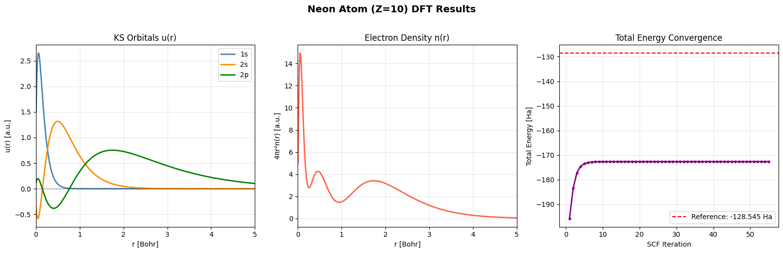
Μετά τη σύγκλιση του αλγορίθμου παράγονται τρία γραφήματα που παρουσιάζουν τα βασικά αποτελέσματα του υπολογισμού.
Τροχιακά Kohn–Sham
Το πρώτο γράφημα απεικονίζει τις ακτινικές κυματοσυναρτήσεις των τροχιακών 1s, 2s και 2p:
$$ u_{1s}(r),\quad u_{2s}(r),\quad u_{2p}(r) $$
Από το διάγραμμα μπορεί να παρατηρηθεί η διαφορετική χωρική κατανομή και ο αριθμός κόμβων κάθε τροχιακού.
Ηλεκτρονιακή Πυκνότητα
Το δεύτερο γράφημα παρουσιάζει την ποσότητα:
$$ 4\pi r^2 n(r) $$
η οποία εκφράζει την πιθανότητα εύρεσης ηλεκτρονίου σε απόσταση \(r\) από τον πυρήνα.
Η καμπύλη αποτυπώνει την κατανομή των δέκα ηλεκτρονίων του νέον γύρω από τον πυρήνα.
Σύγκλιση Ολικής Ενέργειας
Το τρίτο γράφημα παρουσιάζει την εξέλιξη της συνολικής ενέργειας κατά τις επαναλήψεις του SCF:
$$ E_{\mathrm{tot}}^{(1)}, E_{\mathrm{tot}}^{(2)}, E_{\mathrm{tot}}^{(3)}, \dots $$
Παράλληλα εμφανίζεται η βιβλιογραφική τιμή αναφοράς:
$$ E_{\mathrm{ref}} = -128.5450 \;\mathrm{Ha} $$
Η προσέγγιση της υπολογισμένης ενέργειας προς την τιμή αναφοράς αποτελεί ένδειξη της ορθής λειτουργίας του αλγορίθμου και της σύγκλισης της διαδικασίας SCF.
Βιβλιογραφία
David S. Sholl, Janice A. Steckel, Density Functional Theory: A Practical Introduction, 2009, Wiley.
Diouf, Y., Talla, K., Diallo, S., & Gomis, L. (2021). Numerical study of density functional theory of multi-electronic atoms: Case of carbon and helium. American Journal of Nanomaterials, 9(1), 12–22. https://doi.org/10.12691/ajn-9-1-2
Perdew, J. P., & Zunger, A. (1981). Self-interaction correction to density-functional approximations for many-electron systems. Physical Review B, 23(10), 5048–5079. https://doi.org/10.1103/PhysRevB.23.5048